There are three techniques usually used to deal with missing values:
Ignore them and just use complete cases. This is acceptable if <5% of cases are incomplete and missingness is random (Azur, 2004)
Impute values with their mean, median, or mode. A mean imputation leaves the overall mean unchanged, but artificially reduces the variable’s variance (Alice, 2018).
Impute values with multivariate imputation by chained equations (MICE). This method creates multiple predictions of each missing value, allowing the researcher to account for uncertainty in the imputations.
This tutorial explains how to implement MICE using the mice R package.
How MICE works
MICE is a multiple imputation technique. It assumes missing values are “missing at random”, meaning that after controlling for all the variables in the data, any remaining missingingness is completely random. If the data fails this assumption, MICE produces biased estimates.
MICE works by fitting a series of regression models of each variable conditioned on the other variables. The “chained equations” aspect of MICE is four steps.
- Impute simple placeholder values for all missing data (e.g., using the variable mean).
- For each variable with missing values, remove its placeholder values, fit a regression model conditioned on the other data variables, then use the model to replace the missing values with the model predictions.
- Repeat step 2) for a number of cycles, usually 5, each cycle replacing the missing values with improved estimates. By the last cycle, the imputations should be stable.
The “multiple” aspect of MICE is repeating the procedure multiple times, usually 5, to produce a range of imputed values. From this set of values, the researcher can either choose one (the complete() function in mice defaults to choosing the first data set), or pooling the imputations.
Important Considerations
Only include variables that are either in your analysis model (including the response variable) or that are related to the variables that will receive imputations. E.g., if you are imputing height, then exclude subject surname from the MICE procedure. If your analysis model includes interaction terms, include them as well. The MICE model should be more general than your model.
If a variable can be constructed from other variables, then impute the other variable values instead of the summary variable. E.g., body mass index (BMI) is a summary of height and weight. If you have height and weight as variables, impute them then derive BMI rather than imputing BMI directly.
MICE in R
The following case study is based on the vignette’s on the mice package github site. nhanes is a 25x4 data set in the mice package with missing values in several cols.
library(tidyverse)
library(mice)

skimr::skim(nhanes)| Name | nhanes |
| Number of rows | 25 |
| Number of columns | 4 |
| _______________________ | |
| Column type frequency: | |
| numeric | 4 |
| ________________________ | |
| Group variables | None |
Variable type: numeric
| skim_variable | n_missing | complete_rate | mean | sd | p0 | p25 | p50 | p75 | p100 | hist |
|---|---|---|---|---|---|---|---|---|---|---|
| age | 0 | 1.00 | 1.76 | 0.83 | 1.0 | 1.00 | 2.00 | 2.00 | 3.0 | ▇▁▅▁▃ |
| bmi | 9 | 0.64 | 26.56 | 4.22 | 20.4 | 22.65 | 26.75 | 28.92 | 35.3 | ▇▅▆▃▃ |
| hyp | 8 | 0.68 | 1.24 | 0.44 | 1.0 | 1.00 | 1.00 | 1.00 | 2.0 | ▇▁▁▁▂ |
| chl | 10 | 0.60 | 191.40 | 45.22 | 113.0 | 185.00 | 187.00 | 212.00 | 284.0 | ▃▁▇▃▁ |
You might start with an exploration of the missingness pattern. mice::md.pattern() helps you investigate the structure of missing values. The matrix is the missingness pattern (red = missing, blue = not missing). The left column of numbers is the count of instances of the pattern in the data. The right column of numbers is the number of variables in the pattern with missing values (i.e., the number of red boxes). The bottom row of numbers is the count of rows in the data with the number of missing values for the variable. nhanes has 13 rows with complete cases, three rows where only chl is null, etc. chl, hyp, and bmi are simultaneously null 7 times. In all, chl is null 10 times.
mice::md.pattern(nhanes) %>% invisible()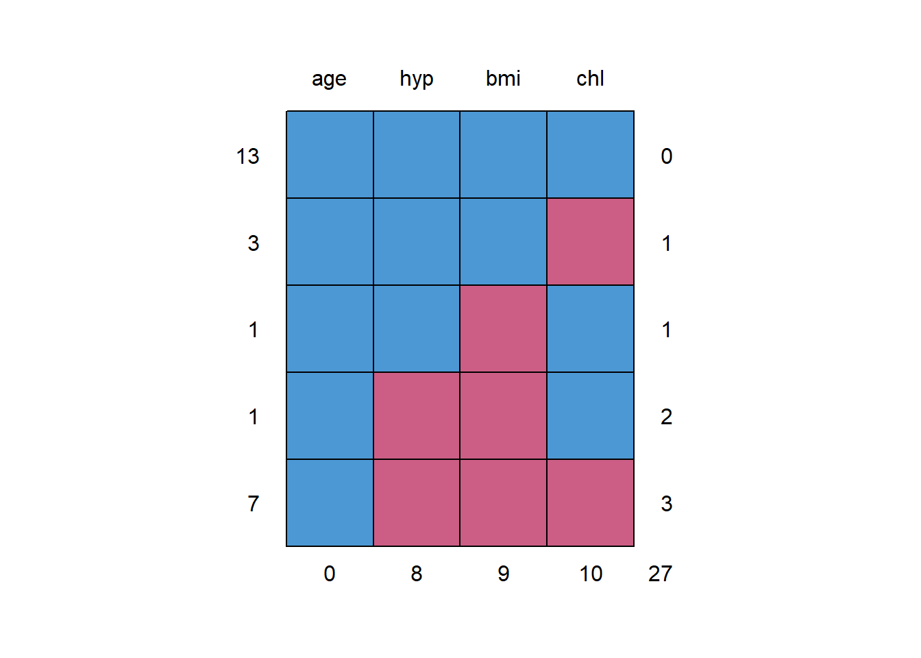
You can simply pass the data frame into mice() to produce the imputations, then complete() to return a new data frame with the missing values replaced by the imputations. mice::mice() returns an object of type multiply imputed data set (mids) that includes the original data, the imputed values, and other metadata. The mice() defaults are to run 5 iterations (maxit = 5) per imputation and m = 5 imputations per missing value. The imputed values are stored as vectors in a list object, imp$imp. Function complete() returns a new data frame with missing values replaced by their imputed value.
imp <- mice::mice(nhanes, print = FALSE, m = 1)

nhanes_2 <- complete(imp)
That’s technically all you have to do, dat %>% mice() %>% complete(). But there are a few things more you should know.
Fine Tune your Analysis
First, you may not want to use all the variables in your data frame to estimate the missing values. E.g., you may have an id column or a character descriptor. You can specify the vars to use with the predctorMatrix parameter and quickpred() utility function. The quickpred() utility function creates a matrix of variables where 1 means it is used in the prediction of the other variable. Below, bmi and hyp are excluded from the list of variables contributing to imputations (although they receive imputed values).
Also, you can set a seed value to guarantee reproducibility.
# What it looks like
quickpred(nhanes, exclude = c("bmi", "hyp"))
## age bmi hyp chl
## age 0 0 0 0
## bmi 1 0 0 1
## hyp 1 0 0 1
## chl 1 0 0 0# In use
imp <- nhanes %>%
mice(
predictorMatrix = quickpred(nhanes, exclude = c("bmi", "hyp")),
print = FALSE,
seed = 123
)You can also evaluate your imputations by inspecting the iteration process to see if the imputed values converged to stable values. The plot() of the mids object shows the mean (left col) and standard deviation (right) col of each variable (rows) imputation iteration. A separate line plot is produced for each imputation. Below you see the 5 iterations (default) along the x-axis and the 5 imputations (default) as colors. The mean bmi ranged from 25-29 in the first iteration and ended at 25-28 by the fifth iteration.
plot(imp)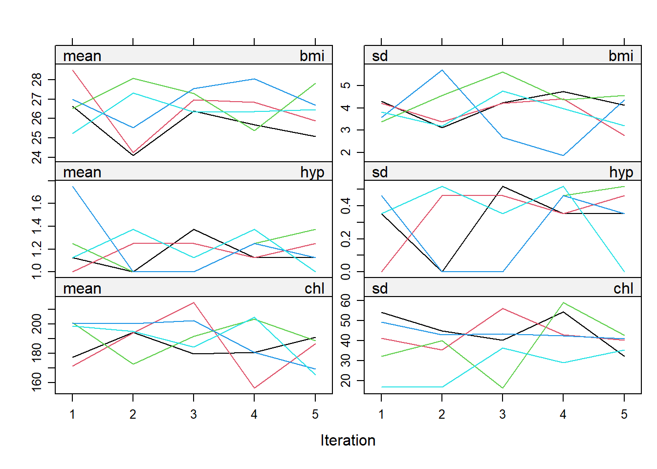
You can produce a density plot to compare the imputation distribution (red) to the non-imputation distribution. They should overlap.
densityplot(imp)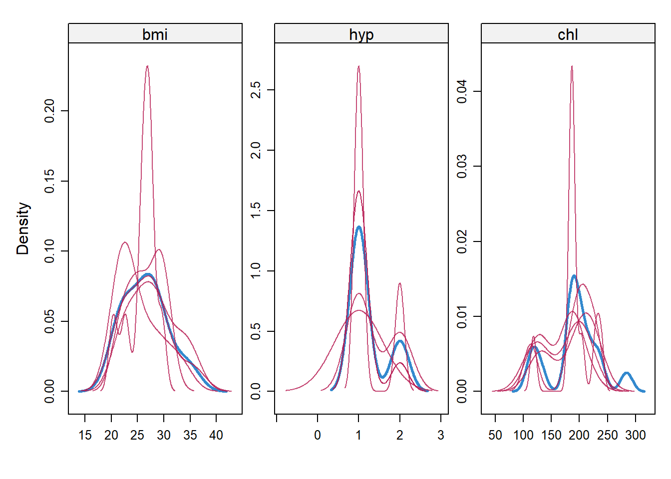
Parting Thoughts
Even though you produce 5 imputations by default, complete() only pulls the first one for you by default. Your can use the others for diagnostics like the plot() above.
The regression model applied to each variable can be independent (OLS for numeric, logistic for binary, Poisson for count, etc.), or even a non-regression model such a classification tree. The mids object returned by mice() tells you which it chose. You can override with the method or defaultMethod parameters.
If you just need a mean or median imputation, mice() can do that for you. Set maxiter = 1 and m = 1 and method = "mean".
imp <- nhanes %>%
  mice(
    m = 1,
    method = "mean",
    maxit = 1,
    print = FALSE
  )
Examples of MICE in action:
References
Azur MJ, Stuart EA, Frangakis C, Leaf PJ. Multiple imputation by chained equations: what is it and how does it work? Int J Methods Psychiatr Res. 2011 Mar;20(1):40-9. doi: 10.1002/mpr.329. PMID: 21499542; PMCID: PMC3074241. html.
Alice, Michy. Imputing Missing Data with R; MICE package. Published Oct 4, 2015, Updated May 14, 2018. html.
mice R package on GitHub with links to vignettes. github
van Buuren, S., & Groothuis-Oudshoorn, K. (2011). mice: Multivariate Imputation by Chained Equations in R. Journal of Statistical Software, 45(3), 1–67. https://doi.org/10.18637/jss.v045.i03. jstatsoft.