Interpreting Logistic Regression Interactions

Odds and Odds Ratios

The esoph dataset is a count of cancer cases in a case-control study. Column ncases is a count of positive diagnoses and ncontrols is a count of negative diagnoses. The dataset has three explanatory variables, but to keep this simple, I’ll narrow the set to one age group, three levels of explanatory variable alcohol consumption (alcgp) and two levels of tobacco consumption (tobgp).

library(tidyverse)

dat <- esoph %>%
  filter(agegp == "65-74") %>%
  mutate(alc = factor(alcgp, ordered = FALSE),
         alc = fct_collapse(alc, 
                            "L" = "0-39g/day", 
                            "M" = "40-79", 
                            "H" = "80-119", "H" = "120+"),
         tob = factor(tobgp, ordered = FALSE),
         tob = fct_collapse(tob, 
                            "L" = "0-9g/day", 
                            "H" = c("10-19", "20-29", "30+"))) %>%
  group_by(alc, tob) %>%
  summarize(.groups = "drop", 
            ncases = sum(ncases), 
            ncontrols = sum(ncontrols))

dat
## # A tibble: 6 x 4
##   alc   tob   ncases ncontrols
##   <fct> <fct>  <dbl>     <dbl>
## 1 L     L          5        43
## 2 L     H          6        17
## 3 M     L         17        17
## 4 M     H          8        11
## 5 H     L          9         8
## 6 H     H         10        10

The cancer odds is the ratio of the probability of a positive diagnosis to the probability of a negative diagnosis, which given the common denominator is just the ratio of counts.

\[odds = \frac{\pi_+}{\pi_-} = \frac{\mathrm{ncases / n}}{\mathrm{ncontrols / n}} = \frac{\mathrm{ncases}}{\mathrm{ncontrols}}\]

dat <- dat %>%
  mutate(odds = ncases / ncontrols)

dat %>% 
  ggplot(aes(x = tob, y = odds, color = alc, group = alc)) +
  geom_point(stat = "summary", fun = sum) +
  stat_summary(fun = sum, geom="line") +
  geom_label(aes(label = scales::number(odds, accuracy = .001))) +
  labs(title = "Alcohol moderates effect of tobacco on cancer odds.") +
  theme_light()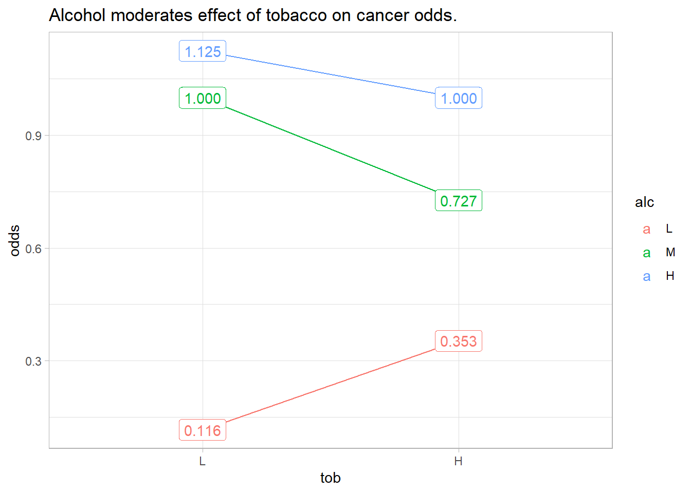

The figure above shows how cancer odds increase with tobacco use and with alcohol consumption, but their effects vary by their combination. If tobacco and alcohol had independent effects on cancer, you’d see parallel lines. Instead, we say alcohol “moderates” the effect of tobacco on cancer risk, and vice-versa.

You can combine these six combinations of alcohol and tobacco into odds ratios (OR). There are 6x6=36 possible ORs. In my experience, I’ve only cared about comparisons to the reference group. From the data frame definition, we’ve chosen tob = “L” and alc = “L” as the reference group. Its the top row in Table 1.

odds_ratios <- merge(dat, dat, by = NULL) %>%
  mutate(odds_1_lbl = paste0("alc", alc.x, "tob", tob.x),
         odds_2_lbl = paste0("alc", alc.y, "tob", tob.y),
         odds_ratio_lbl = paste(odds_1_lbl, odds_2_lbl, sep = ":"),
         OR = odds.x / odds.y) %>%
  select(odds_1_lbl, odds_2_lbl, odds_ratio_lbl, odds_1 = odds.x, odds_2 = odds.y, OR)

odds_ratios %>% 
  mutate(odds_1 = scales::number(odds_1, accuracy = .001),
         odds_2 = scales::number(odds_2, accuracy = .001),
         OR = scales::number(OR, accuracy = .001),
         ` ` = paste(odds_1_lbl, odds_1)) %>%
  select(-c(odds_ratio_lbl, odds_1_lbl, odds_1)) %>%
  pivot_wider(names_from = c(odds_2_lbl, odds_2), values_from = OR, names_sep = "\n") %>%
  flextable::flextable() %>%
  flextable::set_caption("36 possible odds ratios formed from 6 odds.") %>%
  flextable::theme_vanilla() %>%
  flextable::border(j = 1, border.right = officer::fp_border()) %>%
  flextable::bold(j = 1) %>%
  flextable::autofit()

Logistic Regression Model

Recall that a logistic regression fits the log odds of the response variable to the predictor variables. In the equation below, \(\pi\) is the event probability (in this case, a cancer diagnosis).

\[y = \mathrm{logit(\pi)} = \ln\left(\frac{\pi}{1-\pi}\right) = X\beta\]

Our data set is summarized so that ncases and ncontrols combine to specify the binary response to the predictor combinations (see ?glm()). Let’s model the log-odds of cancer as a function of alcohol and tobacco consumption, including their interaction.

mdl <- glm(cbind(ncases, ncontrols) ~ alc*tob, data = dat, 
           family = binomial())

broom::tidy(mdl)
## # A tibble: 6 x 5
##   term        estimate std.error statistic    p.value
##   <chr>          <dbl>     <dbl>     <dbl>      <dbl>
## 1 (Intercept)    -2.15     0.472     -4.55 0.00000526
## 2 alcM            2.15     0.584      3.69 0.000228  
## 3 alcH            2.27     0.678      3.35 0.000812  
## 4 tobH            1.11     0.670      1.66 0.0974    
## 5 alcM:tobH      -1.43     0.884     -1.62 0.106     
## 6 alcH:tobH      -1.23     0.941     -1.31 0.192

The intercept term, -2.152, is the log odds of a positive cancer diagnosis for the reference group (tob = “L” and alc = “L”). The p-value is <.0001, so it is significantly different from 0. Its exponential, 0.116, equals \(e^\hat{Y}\), the odds of a positive cancer diagnosis for the reference group. That means a tob = “L”, alc = “L” person has an expected probability of cancer of \(e^\hat{Y} / (1 + e^\hat{Y}) =\) 10.4% (inverse logit formula).

The interpretation of the coefficient estimators, \(\hat{\beta}\), is “a \(\delta\) change in x is associated with a \(\delta\hat{\beta}\) change in the log-odds of y.” A difference in logs is the same as the log of their ratio, so you can express the change as a ratio.

\[\begin{eqnarray} \delta\beta &=& \log(\pi / (1-\pi))|_{X_1} - \log(\pi / (1-\pi))|_{X_0}\\ &=& \log\left[\frac{\pi / (1-\pi)|_{X_1}}{\pi / (1-\pi)|_{X_0}}\right] \end{eqnarray}\]

A \(\delta = 1\) unit increase in tobH from 0 to 1 (from “L” to “H”) is associated with a 1.11 increase in the log-odds of cancer for a low-alcohol (alc = “L”) user. Log-odds are abstract, but since we can express the change in log-odds as the log of a ratio, we can take the exponential.

\[e^{\delta\beta} = \frac{\pi / (1-\pi)|_{X_1}}{\pi / (1-\pi)|_{X_0}} = \mathrm{OR}\]

The exponentiated coefficient estimators equal the ratio of the odds after and before the change. I.e., they are odds ratios. A \(\delta\) unit change in x is associated with a factor \(e^{\delta\hat{\beta}}\) change in the odds of y.

broom::tidy(mdl, exponentiate = TRUE)

## # A tibble: 6 x 5
##   term        estimate std.error statistic    p.value
##   <chr>          <dbl>     <dbl>     <dbl>      <dbl>
## 1 (Intercept)    0.116     0.472     -4.55 0.00000526
## 2 alcM           8.60      0.584      3.69 0.000228  
## 3 alcH           9.67      0.678      3.35 0.000812  
## 4 tobH           3.04      0.670      1.66 0.0974    
## 5 alcM:tobH      0.240     0.884     -1.62 0.106     
## 6 alcH:tobH      0.293     0.941     -1.31 0.192

We’ve just seen that the exponential of the intercept, exp(tobH) = 0.116, is the odds of a positive cancer diagnosis for the reference group (alc = L, tob = L). Now look at the three main-effects terms, alcM, alcH, and tobH. These terms are the expected change in the log odds of a positive cancer diagnosis associated with a \(\delta = 1\) unit change in the variable holding the other variable at the reference level. E.g., alcM is the change in the log odds associated with a tob = L person changing from alc = L to alc = M. The log of a difference equals the ratio of the logs (basic math), so the exponential of the alcM, alcH, and tobH is the ratio of the odds, the odds ratio (OR).

• alcM = 8.60 is the odds of a positive diagnosis for alc = M, tob = L over the odds of a positive diagnosis for alc = L tob = L.
  
• alcH = 9.67 is the odds of a positive diagnosis for alc = H, tob = L over the odds of a positive diagnosis for alc = L tob = L.
  
• tobH = 3.04 is the odds of a positive diagnosis for alcL = L, tob = H over the odds of a positive diagnosis for alc = L tob = L.

Interaction Effects

Now we’re ready to tackle the interaction terms. The interaction terms measure the incremental change in the odds when you hold the other variable fixed at a different level. E.g., when estimating the change in the log odds of a positive diagnosis associated with a change from alc = L to alc = M, alcM:tobH is the adjustment associated with using a reference level tob = H instead of tob = H.

• alcM * alcM:tobH = 8.60 * 0.24 = 2.06 is the odds of a positive diagnosis for alc = M, tob = H over alc = L tob = H.
• tobH * alcM:tobH = 3.04 * 0.24 = 0.73 is the odds of a positive diagnosis for alc = M, tob = H over alc = M tob = L.
• alcH * alcH:tobH = 9.67 * 0.29 = 2.83 is the odds of a positive diagnosis for alc = H, tob = H over alc = L tob = H.
• tobH * alcH:tobH = 3.04 * 0.29 = 0.89 is the odds of a positive diagnosis for alc = H, tob = H over alc = H tob = L.

But wait - there’s two more odds ratios we can estimate! The effects are multiplicative, so we can calculate the odds ratios of changing both alc and tob vs the reference group.

• alcM * tobH * alcM:tobH = 8.60 * 3.04 * 0.24 = 6.25 is the odds of a positive diagnosis for alc = M, tob = H over alc = L tob = L.
• alcH * tobH * alcH:tobH = 9.67 * 3.04 * 0.29 = 8.60 is the odds of a positive diagnosis for alc = H, tob = H over alc = L tob = L.

If you are following along, you see we’ve calculated 7 of the odds ratios from Table 1. In fact, you can calculate all 36 odds ratios through combinations of main effects and interaction effects.

alcLtobL = exp(coef(mdl)["(Intercept)"])
alcLtobH = exp(coef(mdl)["tobH"])
alcMtobL = exp(coef(mdl)["alcM"])
alcMtobH = exp(coef(mdl)["alcM"]) * exp(coef(mdl)["tobH"]) * exp(coef(mdl)["alcM:tobH"])
alcHtobL = exp(coef(mdl)["alcH"])
alcHtobH = exp(coef(mdl)["alcH"]) * exp(coef(mdl)["tobH"]) * exp(coef(mdl)["alcH:tobH"])
tribble(
  ~num, ~den, ~OR,
  "alcLtobL", "1", alcLtobL,
  "alcLtobH", "1", alcLtobL * alcLtobH,
  "alcMtobL", "1", alcLtobL * alcMtobL,
  "alcMtobH", "1", alcLtobL * alcMtobH,
  "alcHtobL", "1", alcLtobL * alcHtobL,
  "alcHtobH", "1", alcLtobL * alcHtobH,
  "alcLtobL", "alcLtobL", exp(coef(mdl)["(Intercept)"]) / exp(coef(mdl)["(Intercept)"]),
  "alcLtobH", "alcLtobL", alcLtobH,
  "alcMtobL", "alcLtobL", alcMtobL,
  "alcMtobH", "alcLtobL", alcMtobH,
  "alcHtobL", "alcLtobL", alcHtobL,
  "alcHtobH", "alcLtobL", alcHtobH,
  "alcLtobL", "alcLtobH", 1 / alcLtobH,
  "alcLtobH", "alcLtobH", alcLtobH / alcLtobH,
  "alcMtobL", "alcLtobH", alcMtobL / alcLtobH,
  "alcMtobH", "alcLtobH", alcMtobH / alcLtobH,
  "alcHtobL", "alcLtobH", alcHtobL / alcLtobH,
  "alcHtobH", "alcLtobH", alcHtobH / alcLtobH,
  "alcLtobL", "alcMtobL", 1 / alcMtobL,
  "alcLtobH", "alcMtobL", alcLtobH / alcMtobL,
  "alcMtobL", "alcMtobL", alcMtobL / alcMtobL,
  "alcMtobH", "alcMtobL", alcMtobH / alcMtobL,
  "alcHtobL", "alcMtobL", alcHtobL / alcMtobL,
  "alcHtobH", "alcMtobL", alcHtobH / alcMtobL,
  "alcLtobL", "alcMtobH", 1 / alcMtobH,
  "alcLtobH", "alcMtobH", alcLtobH / alcMtobH,
  "alcMtobL", "alcMtobH", alcMtobL / alcMtobH,
  "alcMtobH", "alcMtobH", alcMtobH / alcMtobH,
  "alcHtobL", "alcMtobH", alcHtobL / alcMtobH,
  "alcHtobH", "alcMtobH", alcHtobH / alcMtobH,
  "alcLtobL", "alcHtobL", 1 / alcHtobL,
  "alcLtobH", "alcHtobL", alcLtobH / alcHtobL,
  "alcMtobL", "alcHtobL", alcMtobL / alcHtobL,
  "alcMtobH", "alcHtobL", alcMtobH / alcHtobL,
  "alcHtobL", "alcHtobL", alcHtobL / alcHtobL,
  "alcHtobH", "alcHtobL", alcHtobH / alcHtobL,
  "alcLtobL", "alcHtobH", 1 / alcMtobH,
  "alcLtobH", "alcHtobH", alcLtobH / alcHtobH,
  "alcMtobL", "alcHtobH", alcMtobL / alcHtobH,
  "alcMtobH", "alcHtobH", alcMtobH / alcHtobH,
  "alcHtobL", "alcHtobH", alcHtobL / alcHtobH,
  "alcHtobH", "alcHtobH", alcHtobH / alcHtobH
) %>%
  pivot_wider(names_from = num, values_from = OR) %>%
  flextable::flextable() %>%
  flextable::set_caption("Odds ratios calculated from regression coefficients.") %>%
  flextable::theme_vanilla() %>%
  flextable::border(j = 1, border.right = officer::fp_border()) %>%
  flextable::bold(j = 1) %>%
  flextable::colformat_double(digits = 3) %>%
  flextable::autofit()

About the p-Values

Neither of the interaction term p-values were significant at the .05 level. That means the slopes of the moderation lines are not significantly different from the reference levels line.

If neither interaction term is significant, that means it was unnecessary to control for the interaction in the model. The main effect is the same at all levels of the controlling variables.

If an interaction term is significant, but the main effect is not significant, it means the combined effects differ from the reference group, but changing only one variable is not different from the reference group. In our example, it would mean alcM & tobH differs alc = “L” and tob = “L”, but not from either alcL & tobH or alcM & tobL.

If both the main effect and the interaction effect is significant, it means you must interpret your results relative to the reference group.

This raises another question. How do you report the p-value of the combined effect of two or more coefficients? The theoretical answer is that you need to combine the coefficient estimate variances to calculate a new t-statistic. Say you fit a model

\[ y = \beta_0 + \beta_1 \mathrm{alc} + \beta_2 \mathrm{tob} + \beta_3 \mathrm{alc:tob} + \epsilon \]

and your fitted model coefficient estimators include \(\hat{\beta}_{1M}\) (Medium Alcohol), \(\hat{\beta}_{2H}\) (High Tobacco), and \(\hat{\beta}_{3MH}\) (MediumAlcohol:HighTobacco). The estimator for the combined effect of Medium Alcohol & High Tobacco relative to the reference group Low Alcohol & Low Tobacco, \(\hat{\alpha}\), is \(\hat{\alpha} = \hat{\beta}_{1M} + \hat{\beta}_{2H} + \hat{\beta}_{3MH}\). The p-value associated with \(\hat{\alpha}\) is \(p = P(T>t)\) where \(t = \hat{\alpha} / \mathrm{SE}(\hat{\alpha})\) (same as for any coefficient estimator). The difficulty is in retrieving \(\mathrm{SE}(\hat{\alpha})\). It equals the squre root of te cobined coefficient estimator variances (Wikipedia), \(\mathrm{SE}(\alpha) = \sqrt{\mathrm{Var}(\alpha)}\):

\[ \begin{aligned} \mathrm{Var}(\alpha) = {} & \mathrm{Var}(\hat{\beta}_{1M}) + \mathrm{Var}(\hat{\beta}_{2H}) + \mathrm{Var}(\hat{\beta}_{3HM}) + \\ & 2 \left(\mathrm{Cov}(\hat{\beta}_{1M}\hat{\beta}_{2H}) + \mathrm{Cov}(\hat{\beta}_{1M}\hat{\beta}_{3MH} + \mathrm{Cov}(\hat{\beta}_{2H}\hat{\beta}_{3MH}))\right) \end{aligned} \]

Let’s see this calculation by taking elements from the model variance-covariance matrix.

mdl_vcov <- mdl %>% vcov() %>%  data.frame() %>% rownames_to_column()

var_alcM <- mdl_vcov %>% filter(rowname == "alcM") %>% pull("alcM")
var_tobH <- mdl_vcov %>% filter(rowname == "tobH") %>% pull("tobH")
var_alcMtobH <- mdl_vcov %>% filter(rowname == "alcM:tobH") %>% pull("alcM.tobH")
cov_alcM_tobH <- mdl_vcov %>% filter(rowname == "alcM") %>% pull("tobH")
cov_alcM_alcMtobH <- mdl_vcov %>% filter(rowname == "alcM") %>% pull("alcM.tobH")
cov_tobH_alcMtobH <- mdl_vcov %>% filter(rowname == "tobH") %>% pull("alcM.tobH")

# alpha
(alpha <- coef(mdl)["alcM"] + coef(mdl)["tobH"] + coef(mdl)["alcM:tobH"])
##     alcM 
## 1.833308

# SE for Medium Alcohol + High Tobacco
(se <- sqrt(var_alcM + var_tobH + var_alcMtobH + 
             2 * (cov_alcM_tobH + cov_alcM_alcMtobH + cov_tobH_alcMtobH)))
## [1] 0.6626948

# t
(t <- alpha / se)
##     alcM 
## 2.766445

# p-value
(p_value <- pt(abs(t), Inf, lower.tail = FALSE)* 2)
##        alcM 
## 0.005667121

Happily, there is a package emmeans that calculates both the combined coefficient effects, and these p-values.

emm <- emmeans::emmeans(mdl, ~ alc * tob)

emm_contrast <- emmeans::contrast(emm, method = "revpairwise", adjust = "none")

emm_contrast %>%
  as_tibble() %>%
  filter(str_detect(contrast, "L L$"))

## # A tibble: 5 x 6
##   contrast  estimate    SE    df z.ratio  p.value
##   <chr>        <dbl> <dbl> <dbl>   <dbl>    <dbl>
## 1 M L - L L     2.15 0.584   Inf    3.69 0.000228
## 2 H L - L L     2.27 0.678   Inf    3.35 0.000812
## 3 L H - L L     1.11 0.670   Inf    1.66 0.0974  
## 4 M H - L L     1.83 0.663   Inf    2.77 0.00567 
## 5 H H - L L     2.15 0.651   Inf    3.31 0.000942

There it is, second from bottom.

Key Take-aways

What have we learned?

• Exponentiated coefficient estimates are odds ratios. The interaction effects are multiplicative moderators of the main effects.

• When the p-value of an interaction is significant, that means the slopes of the odds lines in your figure are statistically different from each other.

• Combinations of main-effects and interaction effects always get you a comparison of one group vs another group.

• Use the emmeans package to calculate odds ratios and their associated p-values.