William Poundstone’s Rock Breaks Scissors (Amazon) shows how people are often predictable in their efforts to be random. For instance, from the title, a good strategy for playing Rocks, Paper, Scissors is to start with paper because your opponent is likely to lead with the aggressive rock. The insights are neat throughout, but I’m especially delighted with the simple applications of probability. Let’s play with a few from the chapter on Chapanis’s random number experiment
Chapanis was a noted industrial designer who worked at Bell Labs in the 1950s. His experiment asked students to write a sequence of 2,520 random digits. Chapanis analyzed how random the sequences actually were. I conducted a mini experiment on myself, writing down 300 random numbers before succumbing to tedium.
chapanis <- str_c(
  "19654378094657264109869482380864380216091452609914526179532427948267049319418",
  "648091694823753689014549318621563892675943217458272872395417642800142238774519",
  "632514589321792045916134219574162598769412430289014826723940183921825732087428",
  "3109924132384210891423614279413976455277149716169314281753649812435"
)
If the sequence is random, the digit frequencies should have a binomial distribution with p = 1/10. You expect noise, but this is too much noise.
tibble(num = 0:9, n = str_count(chapanis, as.character(c(0:9)))) %>%
  mutate(p = n / sum(n)) %>%
  ggplot(aes(x = num, y = p)) +
  geom_col() +
  geom_text(aes(label = n), nudge_y = -.01, color = "white") +
  scale_x_continuous(breaks = 0:9) +
  scale_y_continuous(labels = percent_format()) +
  geom_hline(yintercept = .10, linetype = 2)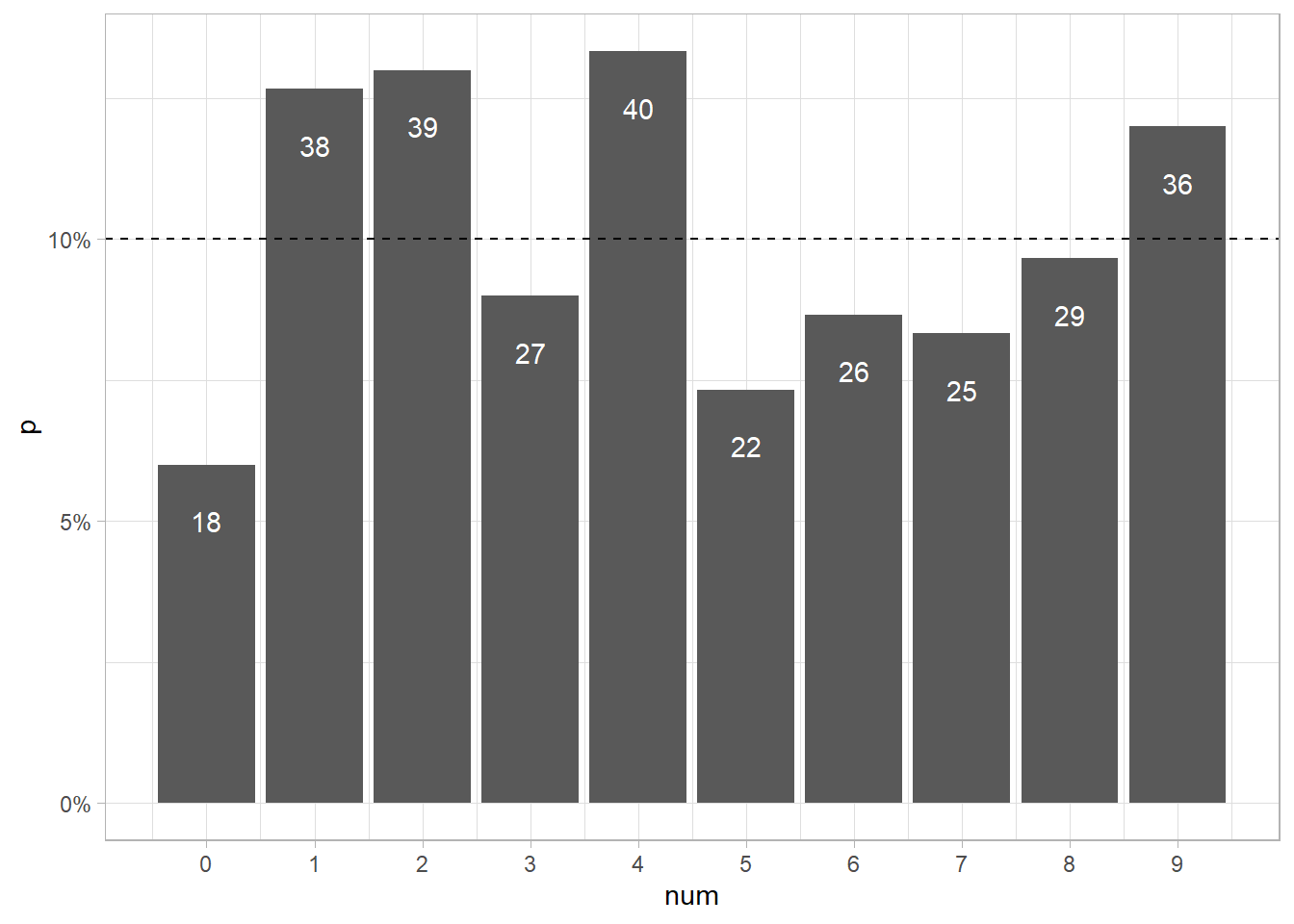
Look at digit 0. I wrote it only 18 times (6%). The expected value is 30 (10%). Astonishingly, the least chosen digit by just about everyone in Chapanis’s study was 0 - even the way I was non-random was non-random! The probability of writing only 18 zeros in a sequence of 300 digits is <1%.
pbinom(q = 18, size = 300, prob = 1/10)## [1] 0.009712619If I really chose digits randomly, 95% of experiments like this would yield between 20 and 41 zeros, so I’m on the tail, but to far down it.
qbinom(p = c(.025, .975), size = 300, prob = 1/10)## [1] 20 41It gets better. Chapanis noticed predictable sequences of numbers too. Participants were unlikely to repeat numbers back to back presumably because that feels non-random. On the other hand, descending sequences like “32” and “21” were over-used. Was that true for me?
# Convert my 300 digit string into a list of 299 2-digit strings.
my_pairs <- map_chr(1:(str_length(chapanis)-1), ~str_sub(chapanis, ., . + 1))

# Frequencies of 2-digit combinations, including combinations I didn't use.
my_freq <- tibble(
  digit_pairs = str_pad(as.character(0:99), 2, "left", "0"),
  freq = map_dbl(digit_pairs, ~sum(my_pairs == .))
  )
There were 13 pairs of numbers I did not write at all. I didn’t write many zeros, so that accounts for five of the 13, but sure enough, five repeated digits are in the list.
my_freq %>% filter(freq == 0) %>% pull(digit_pairs)## [1] "03" "05" "06" "07" "11" "29" "33" "44" "47" "50" "66" "85" "88"Only 7 of my 13 most frequently written pairs were descending.
my_freq %>%
  mutate(
    d1 = str_sub(digit_pairs, 1, 1),
    d2 = str_sub(digit_pairs, 2, 2),
    comp = case_when(d1 > d2 ~ "Descending", d1 < d2 ~ "Ascending", TRUE ~ "Repeating")
  ) %>%
  summarize(.by = comp, freq = sum(freq)) %>%
  mutate(pct = freq / sum(freq))
## # A tibble: 3 × 3
## comp freq pct
## <chr> <dbl> <dbl>
## 1 Repeating 7 0.0234
## 2 Ascending 142 0.475
## 3 Descending 150 0.502The distribution differs from the expected 10% repeats, 45% ascending, 45% descending.
chisq.test(x = c(7, 142, 150), p = c(.10, .45, .45))##
## Chi-squared test for given probabilities
##
## data: c(7, 142, 150)
## X-squared = 19.725, df = 2, p-value = 5.208e-05If the digit sequence was random, it should not be possible to predict the next digit in the sequence with more than 1/10 accuracy. However, Chapanis could guess then next digit 17% of the time. Using the prior two digits improved his accuracy to 28%. For me, the prior digit predicted the next digit 22% of the time, and the prior two digits predicted the next digit 31% of the time.
dat <- tibble(y = str_split_1(chapanis, ""), l1 = lag(y, 1), l2 = lag(y, 2)) %>%
  mutate(across(everything(), factor))

multinom_reg() %>%
  set_engine("nnet") %>%
  fit(y ~ l1, data = dat) %>%
  augment(new_data = dat) %>%
  summarize(M = mean(.pred_class == y, na.rm = TRUE))
## # A tibble: 1 × 1
## M
## <dbl>
## 1 0.221multinom_reg() %>%
set_engine("nnet") %>%
fit(y ~ l1 + l2, data = dat) %>%
augment(new_data = dat) %>%
summarize(M = mean(.pred_class == y, na.rm = TRUE))## # A tibble: 1 × 1
## M
## <dbl>
## 1 0.312